The use of multiple respondents in LSAC provides a rich picture of children's lives and development in various contexts. Across the first seven waves of the study, data were collected from:

• parents of the study child:
  • Parent 1 (P1) - defined as the parent who knows the most about the child (not necessarily a biological parent)
  • Parent 2 (P2), if there is one - defined as another person in the household with a parental relationship to the child, or the partner of Parent 1 (not necessarily a biological parent)
  • a parent living elsewhere (PLE), if there is one - a parent who lives apart from Parent 1 but who has contact with the child (not necessarily a biological parent)
• the study child¹
• carers/teachers (depending on the child's age)
• interviewers.

In earlier waves of the study, the primary respondent was the child's Parent 1. In the majority of cases, this was the child's biological mother, but in a small number of families this was someone else who knew the most about the child. Since Wave 2, the K cohort children have answered age-appropriate interview questions and, from Wave 4, they have also answered a series of self-complete questions. The B cohort children answered a short set of interview questions in Wave 4 for the first time. As children grow older, they are progressively becoming the primary respondents of the study.

A variety of data collection methods are used in the study, including:

• face-to-face interviews:
  • on paper
  • by computer-assisted interview (CAI)
• self-complete questionnaires:
  • during interview (paper forms, computer assisted self-interviews (CASI) and audio computer-assisted self-interviews (ACASI))
  • leave-behind paper forms
  • mail-out paper forms
  • internet-based forms
• physical measurements of the child, including height, weight, girth, body fat and blood pressure
• direct assessment of the child's vocabulary and cognition
• time use diaries (TUD)
• computer-assisted telephone interviews (CATI)
• linkage to administrative or outcome data (e.g. Centrelink, Medicare, MySchool).

Sampling and survey design

The sampling unit for LSAC is the study child. The sampling frame for the study was the Medicare Australia (formerly Health Insurance Commission) enrolments database, which is the most comprehensive database of Australia's population, particularly of young children. In 2004, approximately 18,800 children (aged 0-1 or 4-5 years) were sampled from this database, using a two-stage clustered design. In the first stage, 311 postcodes were randomly selected (very remote postcodes were excluded due to the high cost of collecting data from these areas). In the second stage, children were randomly selected within each postcode, with the two cohorts being sampled from the same postcodes.

A process of stratification was used to ensure that the numbers of children selected were roughly proportionate to the total numbers of children within each state/territory, and within the capital city statistical districts versus the rest of each state. The method of postcode selection accounted for the number of children in the postcode; hence, all the potential participants in Australia had an approximately equal chance of selection (about one in 25). See Soloff, Lawrence, and Johnstone (2005) for more information about the study design.

Response rates

The 18,800 families selected were then invited to participate in the study. Of these, 54% of families agreed to take part in the study (57% of B cohort families and 50% of K cohort families). About 35% of families declined to participate (33% of B cohort families and 38% of K cohort families), and 11% of families (10% of B cohort families and 12% of K cohort families) could not be contacted (e.g. because the address was out-of-date or only a post office box address was provided).

This resulted in a nationally representative sample of 5,107 children aged 0-1 and 4,983 children aged 4-5, who were Australian citizens or permanent residents. This Wave 1 sample was then followed up at later waves of the study. Sample sizes and response rates for each of the main waves are presented in Table 13.1.

Notes: This table refers to the numbers of parents who responded at each wave. Percentages based on weighted data using the Wave 6 data release. ^a The available sample excludes those families who opted out of the study between waves. ^b B cohort: different numbers of parents and their children responded at Wave 5 (there were eight cases where a child interview was completed and the main interview with the parents was not). ^c K cohort: different numbers of parents and their children responded at Wave 3 (in one case a parent interview was completed and the interview with the study child was not); Wave 4 (in five cases a child interview was completed and the main interview with the parents was not); and Wave 5 (in four cases a child interview was completed and the main interview with the parents was not).

Sample weights

Sample weights (for the study children) have been produced for the study dataset in order to reduce the effect of bias in sample selection and participant non-response (Cusack & Defina, 2014; Daraganova & Sipthorp, 2011; Misson & Sipthorp, 2007; Norton & Monahan, 2015; Sipthorp & Misson, 2009; Soloff et al., 2005; Soloff, Lawrence, Misson, & Johnstone, 2006). When these weights are used in the analysis, greater weight is given to population groups that are under-represented in the sample, and less weight to groups that are over-represented in the sample. Weighting therefore ensures that the study sample more accurately represents the sampled population.

These sample weights have been used in analyses presented throughout this report. Cross-sectional or longitudinal weights have been used when examining data from more than one wave. Analyses have also been conducted using Stata® svy (survey) commands, which take the clusters and strata used in the study design into account when producing measures of the reliability of estimates.

Overview of statistical methods and terms used in the report

Confidence interval

A confidence interval (CI) is a range of values, above and below a finding, in which the actual value is likely to fall. The CI represents the accuracy of an estimate, and it can take any number of probabilities, with the most common being 95% or 99%. Unless otherwise specified, the analysis in this report uses a 95% confidence level. This means that the confidence interval covers the true value for 95 out of 100 of the outcomes.

In graphs, 95% confidence intervals are shown by the 'I' bars at the top of each column. Where confidence intervals for the groups being compared do not overlap, this indicates that the differences in values are statistically significant at the p < 0.05 level.

Mean

'Mean' is the statistical term used for what is more commonly known as the average - the sum of the values of a data series divided by the number of data points.

Standard deviation

'Standard deviation (SD)' is a statistical term used for variation or variability in a set of values. Lower standard deviations indicate that the values tend to be close to the mean, while higher standard deviations indicate that the values are spread out over a wider range.

Cohen's d

In this report, differences between means were defined as small, medium or large, according to Cohen's d (Cohen, 1988). Cohen's d is calculated according to the following formula:

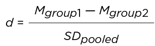
This is the difference in the means of both groups being compared (or mean difference) divided by the pooled standard deviation.

Where:

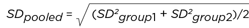
This is the square root of the sum of the standard deviations of both groups being compared divided by two.

A mean difference of d = 0.2 is considered a 'small' effect size, d = 0.5 is considered a 'medium' effect size and d = 0.8 is considered a 'large' effect size (Cohen, 1988).

Odds ratios

An odds ratio (OR) is a measure of association between an exposure and an outcome. The odds ratio represents the odds that an outcome will occur given a particular exposure, compared to the odds of the outcome occurring in the absence of that exposure.

ORs are used to compare the relative odds of the occurrence of the outcome of interest (e.g. disease or disorder), given exposure to the variable of interest (e.g. health characteristic, aspect of medical history). The OR can also be used to determine whether a particular exposure is a risk factor for a particular outcome, and to compare the magnitude of various risk factors for that outcome.

• OR = 1 Exposure does not affect odds of outcome.
• OR > 1 Exposure is associated with higher odds of outcome.
• OR < 1 Exposure is associated with lower odds of outcome.

Logistic regression models

Logistic regression models are used to estimate the effects of factors, such as age and educational attainment, on a categorical dependent variable, such as volunteering status. The standard models examine 'binary' dependent variables, which are variables with only two distinct values, and estimates obtained from these models are interpreted as the effects on the probability that the variable takes one of those values. For example, a model might be estimated on the probability that an individual is volunteering (as opposed to not volunteering).

Chi-square test

A chi-square (X²) test is used to investigate whether distributions of categorical variables differ from one another. For example, are children's worries about the environment different between boys and girls.

Statistical significance

In the context of statistical analysis of survey data, a finding is statistically significant if it is unlikely that the relationship between two or more variables is caused by chance. That is, a relationship can be considered to be statistically significant if we can reject the 'null hypothesis' that hypothesises that there is no relationship between measured variables. A common standard is to regard a difference between two estimates as statistically significant if the probability that they are different is at least 95%. However, 90% and 99% standards are also commonly used. Unless otherwise specified, the 95% standard is adopted for regression results presented in this report. Note that a statistically significant difference does not mean the difference is necessarily large, it simply means that you can be fairly confident there is a difference.

References

Cohen, J. (1988). Statistical power analysis for the behavioral sciences. Hillsdale, N.J.: L. Erlbaum Associates.

Cusack, B., & Defina, R. (2014). Wave 5 weighting & non-response (Technical Paper No. 10). Melbourne: Australian Institute of Family Studies.

Daraganova, G., & Sipthorp, M. (2011). Wave 4 weights (Technical Paper No. 9). Melbourne: Australian Institute of Family Studies.

Misson, S., & Sipthorp, M. (2007). Wave 2 weighting and non-response (Technical Paper No. 5). Melbourne: Australian Institute of Family Studies.

Norton, A., & Monahan, K. (2015). Wave 6 weighting and non-response (Technical Paper No. 15). Melbourne: Australian Institute of Family Studies.

Sipthorp, M., & Misson, S. (2009). Wave 3 weighting and non-response (Technical Paper No. 6). Melbourne: Australian Institute of Family Studies.

Soloff, C., Lawrence, D., & Johnstone, R. (2005). LSAC sample design (Technical Paper No. 1). Melbourne: Australian Institute of Family Studies.

Soloff, C., Lawrence, D., Misson, S., & Johnstone, R. (2006). Wave 1 weighting and non-response. Melbourne: Australian Institute of Family Studies.